Tutorial

1 minute read

Sublime's custom image

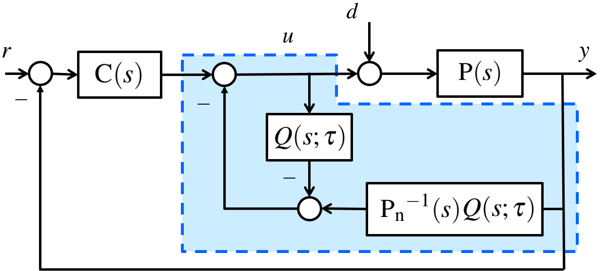
As a tutorial, it is assumed that in the figure,

$C(s) = 2/(s+4)$ ,
$P_n(s) = 5/(s-2)$ ,
$P(s) = \beta_0/(s+\alpha_0)$ , where $4\leq\beta_0\leq 10,\:-10\leq\alpha_0\leq 10$ .

Setup

The following code returns a structure variable sysEnv that contains the information about the system environment that will be used later in designing the DOB.

C = tf(2, [1, 4]);
P_n = tf(5, [1, -2]);

N = {[4, 10]};
D = {1, [-10, 10]};

sysEnv = setup_sys(N, D, P_n, C)

The field nominalStab is 1 since the nominal closed-loop system is stable and the field minPhase is also 1 since a given set of uncertain plants does not contain any non-minimum phase systems (In fact, there is no zero dynamics.).

Design of Q-filter

The following code returns a transfer function model $Q(s;1)$ Qcanon with a constant numerator and the relative degree 3 that robustly stabilizes the fast dynamics of the closed-loop system.

Qcanon = gen_Qcanon(sysEnv, 3)

If you want to try to use your own $Q(s;1)=1/(s+1)$ , the following code informs you if the fast dynamics of the closed-loop system is robustly stable or not.

isFastDynamicsStable(sysEnv, tf(1, [1, 1]))

Finally, the following code returns the supremum $\tau^*$ , supTau such that for all $0<\tau<\tau^*$ , the closed-loop system with the DOB designed under Qcanon is robustly stable. Here, Symbolic Math Toolbox is required for the option 'exact' and 10 means the resolution of the 'approximate' search method.

supTau = get_supTau(sysEnv, Qcanon, 'exact')
supTau = get_supTau(sysEnv, Qcanon, 'approx', 10)

In conclusion, DO-DAT suggests you to use the Q-filter for the robust stability of the closed-loop system as follows.

$Q(s;\tau) = \frac{0.5}{(\tau s)^3+2(\tau s)^2+ (\tau s) + 0.5}$ , for any $0<\tau<0.0232$ .

Twitter Facebook LinkedIn

Tutorial

Setup

Design of Q-filter

You May Also Enjoy

Non-minimum phase case